Advanced usage of BioCor
Lluís Revilla
August Pi i Sunyer Biomedical Research Institute (IDIBAPS); Liver Unit, Hospital Cliniclrevilla@clinic.cat
Juan José Lozano
Centro de Investigación Biomédica en Red de Enfermedades Hepaticas y Digestivas (CIBEREHD); Barcelona, SpainPau Sancho-Bru
August Pi i Sunyer Biomedical Research Institute (IDIBAPS); Liver Unit, Hospital Clinic20 October 2025
Source:vignettes/BioCor_2_advanced.Rmd
BioCor_2_advanced.RmdAbstract
Describes how to use the BioCor package to answer several biological questions and how to use functional similarities with other measures.
Introduction
In this vignette we assume that the reader is already familiarized with the introduction vignette, but wants to know how can it help to answer other questions in other situations
We follow the same convention about names of the objects used
genesReact and genesKegg are the list with
information about the pathways the genes are involved in.
Merging similarities
If one calculates similarities with KEGG data and Reactome or other input for the same genes or clusters BioCor provides a couple of functions to merge them.
We can set a weight to each similarity input with
weighted.sum, multiply them also using a weight for each
similarity (with weighted.prod), doing the mean or just
adding them up. Similarities allow us to apply a function to combine the
matrices of a list. Here we use some of the genes used in the first
vignette:
kegg <- mgeneSim(c("672", "675", "10"), genesKegg)
react <- mgeneSim(c("672", "675", "10"), genesReact)
## We can sum it adding a weight to each origin
weighted.sum(c(kegg["672", "675"], react["672", "675"]), w = c(0.3, 0.7))
## [1] 0.7247289

## Or if we want to perform for all the matrix
## A list of matrices to merge
sim <- list("kegg" = kegg, "react" = react)
similarities(sim, weighted.sum, w = c(0.3, 0.7))
##           672       675        10
## 672 1.0000000 0.7247289 0.1490643
## 675 0.7247289 1.0000000 0.1515368
## 10  0.1490643 0.1515368 1.0000000
similarities(sim, weighted.prod, w = c(0.3, 0.7))
##           672          675           10
## 672 0.2100000 0.0173101952 0.0000000000
## 675 0.0173102 0.2100000000 0.0003685656
## 10  0.0000000 0.0003685656 0.2100000000
similarities(sim, prod)
##           672         675          10
## 672 1.0000000 0.082429501 0.000000000
## 675 0.0824295 1.000000000 0.001755074
## 10  0.0000000 0.001755074 1.000000000
similarities(sim, mean)
##           672       675        10
## 672 1.0000000 0.5412148 0.1064745
## 675 0.5412148 1.0000000 0.1105954
## 10  0.1064745 0.1105954 1.0000000
This functions are similar to weighted.mean, except that
first the multiplication by the weights is done and then the
NAs are removed:
weighted.mean(c(1, NA), w = c(0.5, 0.5), na.rm = TRUE)
## [1] 1
weighted.mean(c(1, 0.5, NA), w = c(0.5, 0.25, 0.25), na.rm = TRUE)
## [1] 0.8333333
weighted.sum(c(1, NA), w = c(0.5, 0.5))
## [1] 0.5
weighted.sum(c(1, 0.5, NA), w = c(0.5, 0.25, 0.25))
## [1] 0.625
weighted.prod(c(1, NA), w = c(0.5, 0.5))
## [1] 0.5
weighted.prod(c(1, 0.5, NA), w = c(0.5, 0.25, 0.25))
## [1] 0.0625
Assessing a differential study
In this example we will use the functional similarities in a classical differential study.
Obtaining data
We start using data from the RNAseq workflow and following the analysis comparing treated and untreated:
suppressPackageStartupMessages(library("airway"))
data("airway")
library("DESeq2")

dds <- DESeqDataSet(airway, design = ~ cell + dex)
dds$dex <- relevel(dds$dex, "untrt")
dds <- DESeq(dds)
## estimating size factors
## estimating dispersions
## gene-wise dispersion estimates
## mean-dispersion relationship
## final dispersion estimates
## fitting model and testing
res <- results(dds, alpha = 0.05)
summary(res)
##
## out of 33469 with nonzero total read count
## adjusted p-value < 0.05
## LFC > 0 (up)       : 2211, 6.6%
## LFC < 0 (down)     : 1817, 5.4%
## outliers [1]       : 0, 0%
## low counts [2]     : 16687, 50%
## (mean count < 7)
## [1] see 'cooksCutoff' argument of ?results
## [2] see 'independentFiltering' argument of ?results
plot(res$log2FoldChange, -log10(res$padj),
    pch = 16, xlab = "log2FC",
    ylab = "-log10(p.ajd)", main = "Untreated vs treated"
)
logFC <- 2.5
abline(v = c(-logFC, logFC), h = -log10(0.05), col = "red")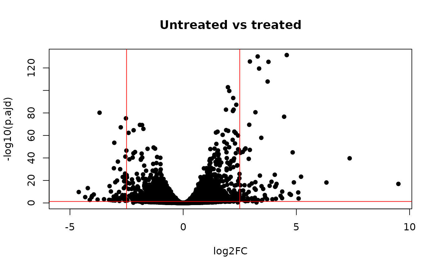
Volcano plot. The airway data
As we can see here there are around 4000 genes differentially expressed genes, some of them differentially expressed above 2^2.5.
Selecting differentially expressed genes
Usually in such a study one selects genes above certain logFC or fold change threshold, here we use the absolute value of 2.5:
fc <- res[abs(res$log2FoldChange) >= logFC & !is.na(res$padj), ]
fc <- fc[fc$padj < 0.05, ]
# Convert Ids (used later)
genes <- select(org.Hs.eg.db,
    keys = rownames(res), keytype = "ENSEMBL",
    column = c("ENTREZID", "SYMBOL")
)
## 'select()' returned 1:many mapping between keys and columns
genesFC <- genes[genes$ENSEMBL %in% rownames(fc), ]
genesFC <- genesFC[!is.na(genesFC$ENTREZID), ]
genesSim <- genesFC$ENTREZID
names(genesSim) <- genesFC$SYMBOL
genesSim <- genesSim[!duplicated(genesSim)]
# Calculate the functional similarity
sim <- mgeneSim(genes = genesSim, info = genesReact, method = "BMA")
## Warning in mgeneSim(genes = genesSim, info = genesReact, method = "BMA"): Some
## genes are not in the list provided.
Once the similarities for the selected genes are calculated we can now visualize the effect of each method:
nas <- apply(sim, 1, function(x) {
    all(is.na(x))
})
sim <- sim[!nas, !nas]

MDSs <- cmdscale(1 - sim)
plot(MDSs, type = "n", main = "BMA similarity", xlab = "MDS1", ylab = "MDS2")
up <- genes[genes$ENSEMBL %in% rownames(fc)[fc$log2FoldChange >= logFC], "SYMBOL"]
text(MDSs, labels = rownames(MDSs), col = ifelse(rownames(MDSs) %in% up, "black", "red"))
abline(h = 0, v = 0)
legend("top", legend = c("Up-regulated", "Down-regulated"), fill = c("black", "red"))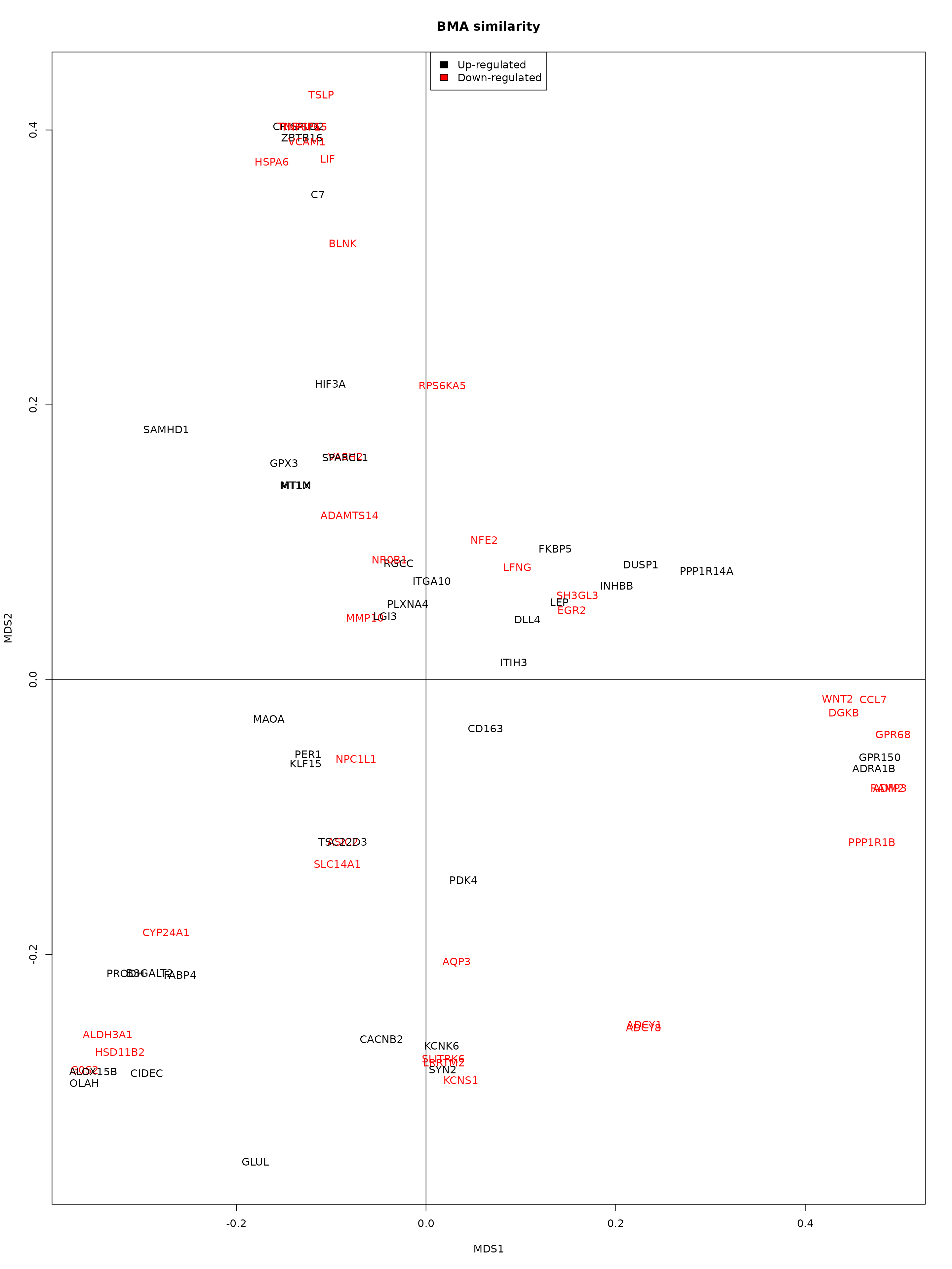
Functional similarity of genes with logFC above 2,5. Similar genes cluster together.
This plot illustrate that some differentially expressed genes are quite similar according to their pathways. Suggesting that there might be a relationship between them. Furthermore, some up-regulated genes seem functionally related to down-regulated genes indicating a precise regulation of the pathways where they are involved.
Note that here we are only using 75 genes from the original 127.
Are differentially expressed genes selected by their functionality?
In the previous section we have seen that some differentially expressed genes are functionally related and that they have a high logFC value. Are genes differentially expressed more functional related than those which aren’t differential expressed?
For simplicity we will use a subset of 400 genes represented again in a volcano plot and we will look for the functional similarities between those genes:
set.seed(250)
subRes <- res[!is.na(res$log2FoldChange), ]
subs <- sample.int(nrow(subRes), size = 400)
subRes <- subRes[subs, ]
g <- genes[genes$ENSEMBL %in% rownames(subRes), "ENTREZID"]
gS <- mgeneSim(g[g %in% names(genesReact)], genesReact, "BMA")
deg <- rownames(subRes[subRes$padj < 0.05 & !is.na(subRes$padj), ])
keep <- rownames(gS) %in% genes[genes$ENSEMBL %in% deg, "ENTREZID"]
plot(subRes$log2FoldChange, -log10(subRes$padj),
    pch = 16, xlab = "log2FC",
    ylab = "-log10(p.ajd)", main = "Untreated vs treated"
)
abline(v = c(-logFC, logFC), h = -log10(0.05), col = "red")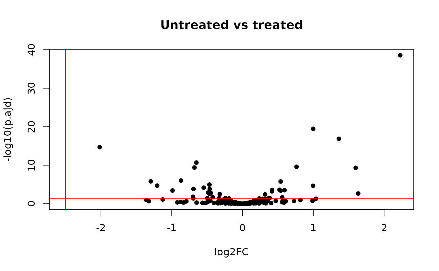
Volcano plot of the subset of 400 genes. This subset will be used in the following sections
We can answer this by testing it empirically:
library("boot")
# The mean of genes differentially expressed
(scoreDEG <- mean(gS[!keep, keep], na.rm = TRUE))
## [1] 0.1203038
b <- boot(data = gS, R = 1000, statistic = function(x, i) {
    g <- !rownames(x) %in% rownames(x)[i]
    mean(x[g, i], na.rm = TRUE)
})
(p.val <- (1 + sum(b$t > scoreDEG)) / 1001)
## [1] 0.6853147
hist(b$t, main = "Distribution of scores", xlab = "Similarity score")
abline(v = scoreDEG, col = "red")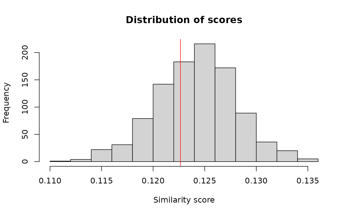
Distribution of scores between differentially expressed genes and those who aren’t. The line indicates the mean score of the similarity between differentially expressed genes and those which aren’t differentially expressed.
Comparing the genes differentially expressed and those who aren’t doesn’t show that they are non-randomly selected (p-value 0.6853147). The genes with a p-value below the threshold are not more closely functionally related than all the other genes1.
Are functionally related the selected differentially expressed genes?
We have seen that the genes differentially expressed aren’t selected by their functionality. However they could be more functionally related than the other genes. Are the differentially expressed genes more functionally similar than it would be expected ?
(scoreW <- combineScores(gS[keep, keep], "avg"))
## [1] 0.1564027
b <- boot(data = gS, R = 1000, statistic = function(x, i) {
    mean(x[i, i], na.rm = TRUE)
})
(p.val <- (1 + sum(b$t > scoreW)) / 1001) # P-value
## [1] 0.005994006
hist(b$t, main = "Distribution of scores", xlab = "Similarity score")
abline(v = scoreW, col = "red")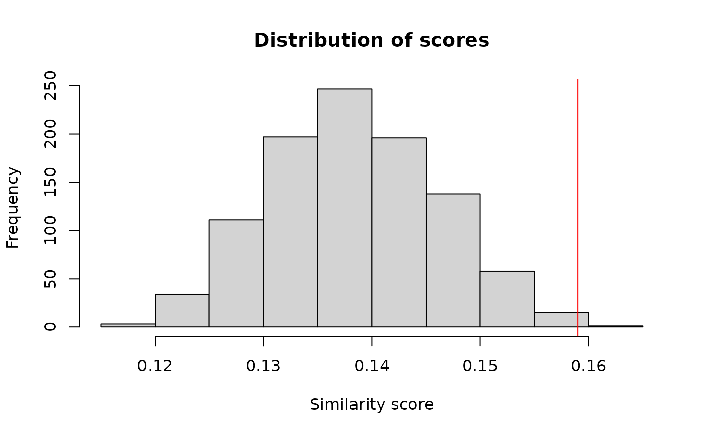
Distribution of the similarity within differentially expressed genes. The line indicates the mean funtional similarity whitin them.
If we selected randomly the genes from our pool we would expect a score around 0.1564027 with a probability of 0.005994. That means that the differentially expressed genes is highly different compared to the other genes if we use a significance threshold of 0.05 2.
Influence of the fold change in the functionally similarity of the genes
We have seen that the genes differentially expressed are not selected by functional similarity but they are functionally related. Now we would like to know if selecting a fold change threshold affects the functional similarity between them.
To know the relationship between the fold change and the similarity between genes we have several methods:
s <- seq(0, max(abs(subRes$log2FoldChange)) + 0.05, by = 0.05)
l <- sapply(s, function(x) {
    deg <- rownames(subRes[abs(subRes$log2FoldChange) >= x, ])
    keep <- rownames(gS) %in% genes[genes$ENSEMBL %in% deg, "ENTREZID"]
    BetweenAbove <- mean(gS[keep, keep], na.rm = TRUE)
    AboveBelow <- mean(gS[keep, !keep], na.rm = TRUE)
    BetweenBelow <- mean(gS[!keep, !keep], na.rm = TRUE)
    c(
        "BetweenAbove" = BetweenAbove, "AboveBelow" = AboveBelow,
        "BetweenBelow" = BetweenBelow
    )
})
L <- as.data.frame(cbind(logfc = s, t(l)))
plot(L$logfc, L$BetweenAbove,
    type = "l", xlab = "abs(log2) fold change",
    ylab = "Similarity score",
    main = "Similarity scores along logFC", col = "darkred"
)
lines(L$logfc, L$AboveBelow, col = "darkgreen")
lines(L$logfc, L$BetweenBelow, col = "black")
legend("topleft",
    legend = c(
        "Between genes above and below threshold",
        "Whitin genes above threshold",
        "Whitin genes below threshold"
    ),
    fill = c("darkgreen", "darkred", "black")
)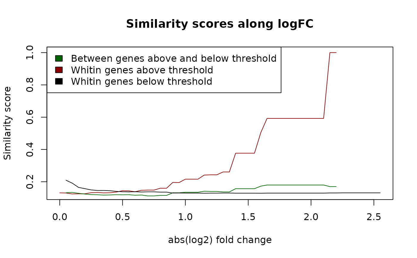
Similarity of genes along abs(logFC). Assessing the similarity of genes according to their absolute log2 fold change.
The functional similarity of the genes above the threshold increases with a more restrictive threshold, indicating that a logFC threshold selects genes by their functionality, or in other words that genes differentially expressed tend to be of related pathways. The similarity between those genes above the threshold and below remains constant as well as within genes below the threshold.
l <- sapply(s, function(x) {
    # Names of genes up and down regulated
    degUp <- rownames(subRes[subRes$log2FoldChange >= x, ])
    degDown <- rownames(subRes[subRes$log2FoldChange <= -x, ])

    # Translate to ids in gS
    keepUp <- rownames(gS) %in% genes[genes$ENSEMBL %in% degUp, "ENTREZID"]
    keepDown <- rownames(gS) %in% genes[genes$ENSEMBL %in% degDown, "ENTREZID"]

    # Calculate the mean similarity between each subgrup
    between <- mean(gS[keepUp, keepDown], na.rm = TRUE)

    c("UpVsDown" = between)
})
L <- as.data.frame(cbind("logfc" = s, "UpVsDown" = l))
plot(L$logfc, L$UpVsDown,
    type = "l",
    xlab = "abs(log2) fold change threshold",
    ylab = "Similarity score",
    main = "Similarity scores along logFC"
)
legend("topright",
    legend = "Up vs down regulated genes",
    fill = "black"
)
Functional similarity between the up-regulated and down-regulated genes.
The maximal functional similarity between genes up-regulated and down-regulated are at 1.15 log2 fold change.
Assessing a new pathway
Sometimes the top differentially expressed genes or some other key
genes are selected as a signature or a potential new group of related
genes. In those cases we can test how does the network of genes change
if we add them. Here we create a new pathway named deg, and
we see the effect on the functional similarity score for all the
genes:
# Adding a new pathway "deg" to those genes
genesReact2 <- genesReact
diffGenes <- genes[genes$ENSEMBL %in% deg, "ENTREZID"]
genesReact2[diffGenes] <- sapply(genesReact[diffGenes], function(x) {
    c(x, "deg")
})
plot(ecdf(mgeneSim(names(genesReact), genesReact)))
curve(ecdf(mgeneSim(names(genesReact2), genesReact2)), color = "red")
This would take lot of time, for a illustration purpose we reduce to some genes:
library("Hmisc")
genesReact2 <- genesReact
diffGenes <- genes[genes$ENSEMBL %in% deg, "ENTREZID"]
# Create the new pathway called deg
genesReact2[diffGenes] <- sapply(genesReact[diffGenes], function(x) {
    c(x, "deg")
})
ids <- unique(genes[genes$ENSEMBL %in% rownames(subRes), "ENTREZID"])
Ecdf(c(mgeneSim(ids, genesReact, method = "BMA"),
       mgeneSim(ids, genesReact2, method = "BMA")
),
group = c(rep("Reactome", length(ids)^2), rep("Modified", length(ids)^2)),
col = c("black", "red"), xlab = "Functional similarities",
main = "Empirical cumulative distribution")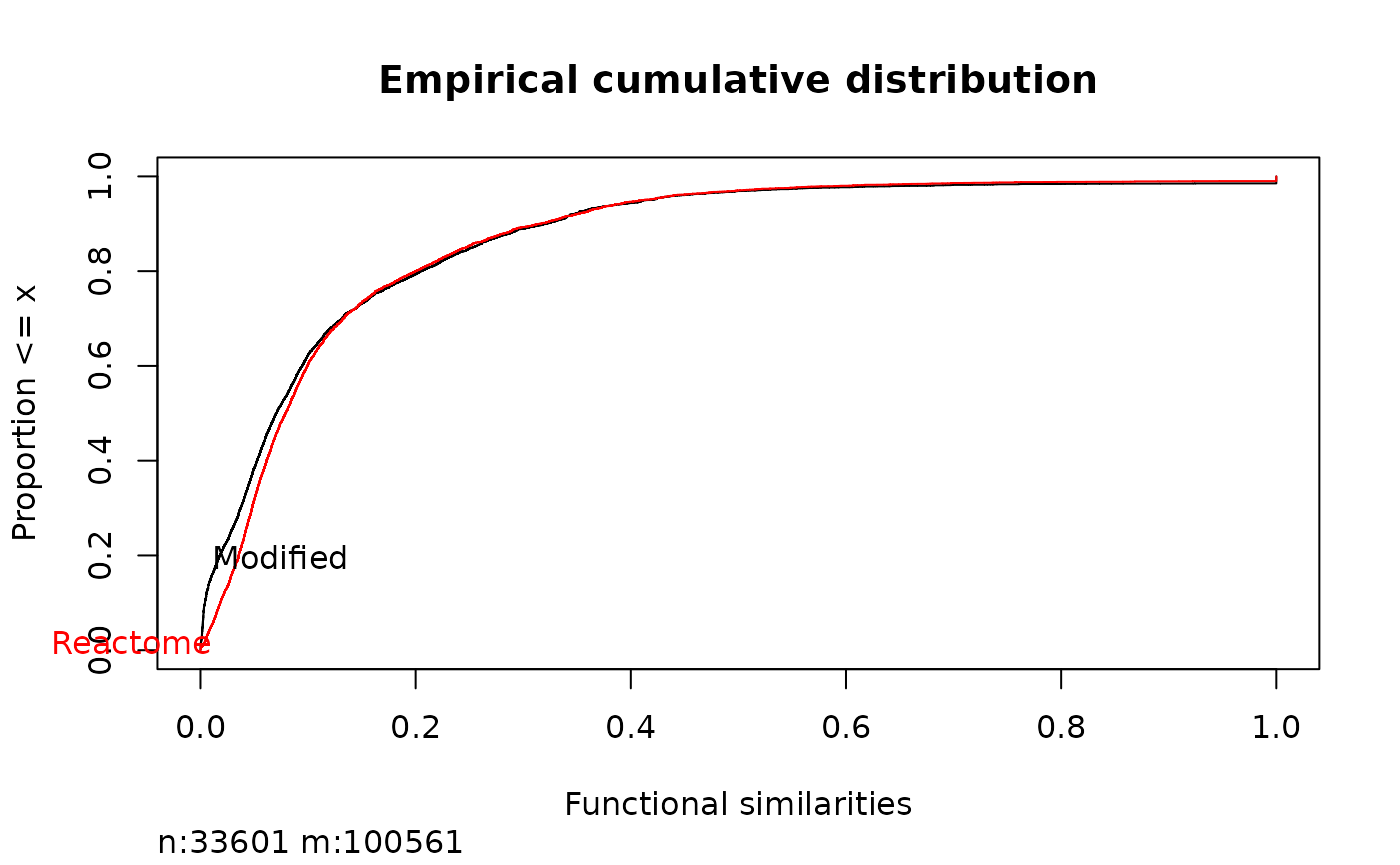
The effect of adding a new pathway to a functional similarity. In red the same network as in black but with the added pathway.
Merging sources of information
Sometimes we have several origin of information, either several
databases, or information from other programs… We can merge this in the
single object required by the function in BioCor using the
function combineSources3.
This functions helps to evaluate what happens when we add more pathway information. For instance here we add the information in Kegg and the information in Reactome and we visualize it using the same procedure as previously:
genesKegg <- as.list(org.Hs.egPATH)
gSK <- mgeneSim(rownames(gS), genesKegg)
mix <- combineSources(genesKegg, genesReact)
## Warning in combineSources(genesKegg, genesReact): More than 50% of genes identifiers of a source are unique
## Check the identifiers of the genes
gSMix <- mgeneSim(rownames(gS), mix)
Ecdf(c(gS, gSK, gSMix),
    group = c(
        rep("Reactome", length(gS)), rep("Kegg", length(gSK)),
        rep("Mix", length(gSMix))
    ),
    col = c("black", "red", "blue"), xlab = "Functional similarities",
    main = "Empirical cumulative distribution."
)
## Warning in regularize.values(x, y, ties, missing(ties), na.rm = na.rm):
## collapsing to unique 'x' values
## Warning in regularize.values(x, y, ties, missing(ties), na.rm = na.rm):
## collapsing to unique 'x' values
## Warning in regularize.values(x, y, ties, missing(ties), na.rm = na.rm):
## collapsing to unique 'x' values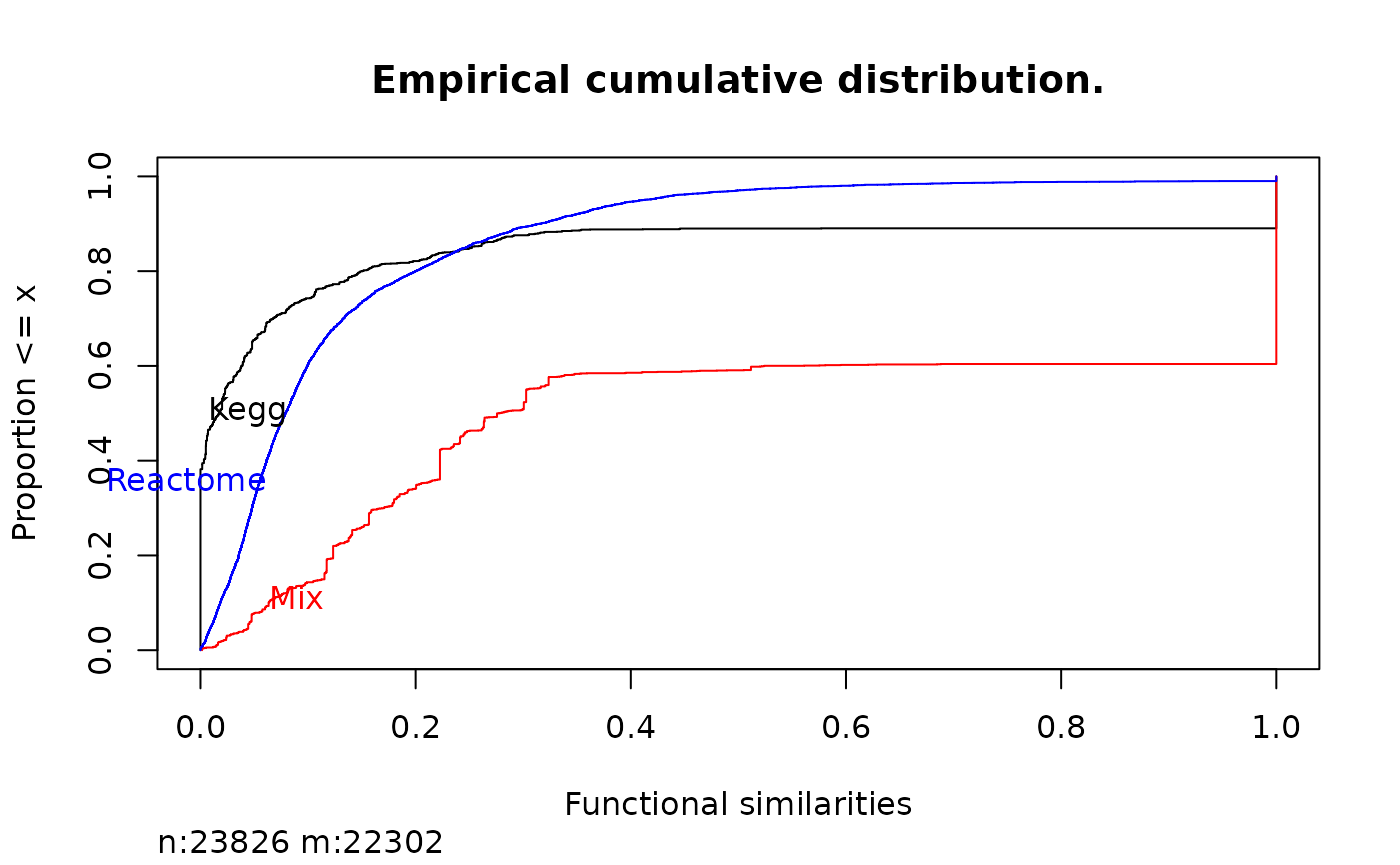
Comparison of functional similarity in different databases.
When mixed, there is a huge increase in the genes that share a
pathway using the max method. Observe in next figure
(@ref(fig:combineSource2)) how does the method affects to the
results:
gSK2 <- mgeneSim(rownames(gS), genesKegg, method = "BMA")
gS2 <- mgeneSim(rownames(gS), genesReact, method = "BMA")
gSMix2 <- mgeneSim(rownames(gS), mix, method = "BMA")
Ecdf(c(gS2, gSK2, gSMix2),
    group = c(
        rep("Reactome", length(gS)), rep("Kegg", length(gSK)),
        rep("Mix", length(gSMix))
    ),
    col = c("black", "red", "blue"), xlab = "Functional similarities (BMA)", main = "Empirical cumulative distribution."
)
## Warning in regularize.values(x, y, ties, missing(ties), na.rm = na.rm):
## collapsing to unique 'x' values
## Warning in regularize.values(x, y, ties, missing(ties), na.rm = na.rm):
## collapsing to unique 'x' values
## Warning in regularize.values(x, y, ties, missing(ties), na.rm = na.rm):
## collapsing to unique 'x' values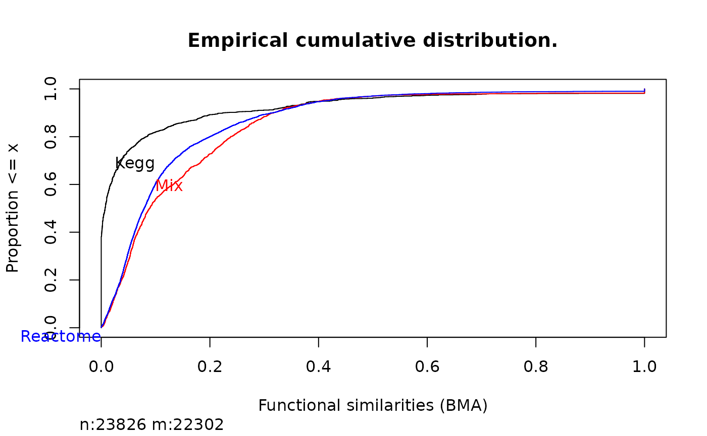
Comparison of functional similarity in different gene sets.
Now we can appreciate that most of the functional similarity is brought by Reactome database
Comparing with GO similarities
As suggested in the main vignette functional similarities can be compared to semantic similarities such as those based on GO. Here a comparison using the biological process from the gene ontologies is done:
library("GOSemSim")
##
## GOSemSim v2.34.0 Learn more at https://yulab-smu.top/contribution-knowledge-mining/
##
## Please cite:
##
## Guangchuang Yu, Fei Li, Yide Qin, Xiaochen Bo, Yibo Wu and Shengqi
## Wang. GOSemSim: an R package for measuring semantic similarity among GO
## terms and gene products. Bioinformatics. 2010, 26(7):976-978
##
## Attaching package: 'GOSemSim'
## The following objects are masked from 'package:BioCor':
##
##     clusterSim, combineScores, geneSim, mclusterSim, mgeneSim
BP <- godata("org.Hs.eg.db", ont = "BP", computeIC = TRUE)
## Warning in godata("org.Hs.eg.db", ont = "BP", computeIC = TRUE): use 'annoDb'
## instead of 'OrgDb'
## preparing gene to GO mapping data...
## preparing IC data...
gsGO <- GOSemSim::mgeneSim(rownames(gS), semData = BP, measure = "Resnik", verbose = FALSE)
keep <- rownames(gS) %in% rownames(gsGO)
hist(as.dist(gS[keep, keep] - gsGO),
    main = "Difference between functional similarity and biological process",
    xlab = "Functional similarity - biological process similarity"
)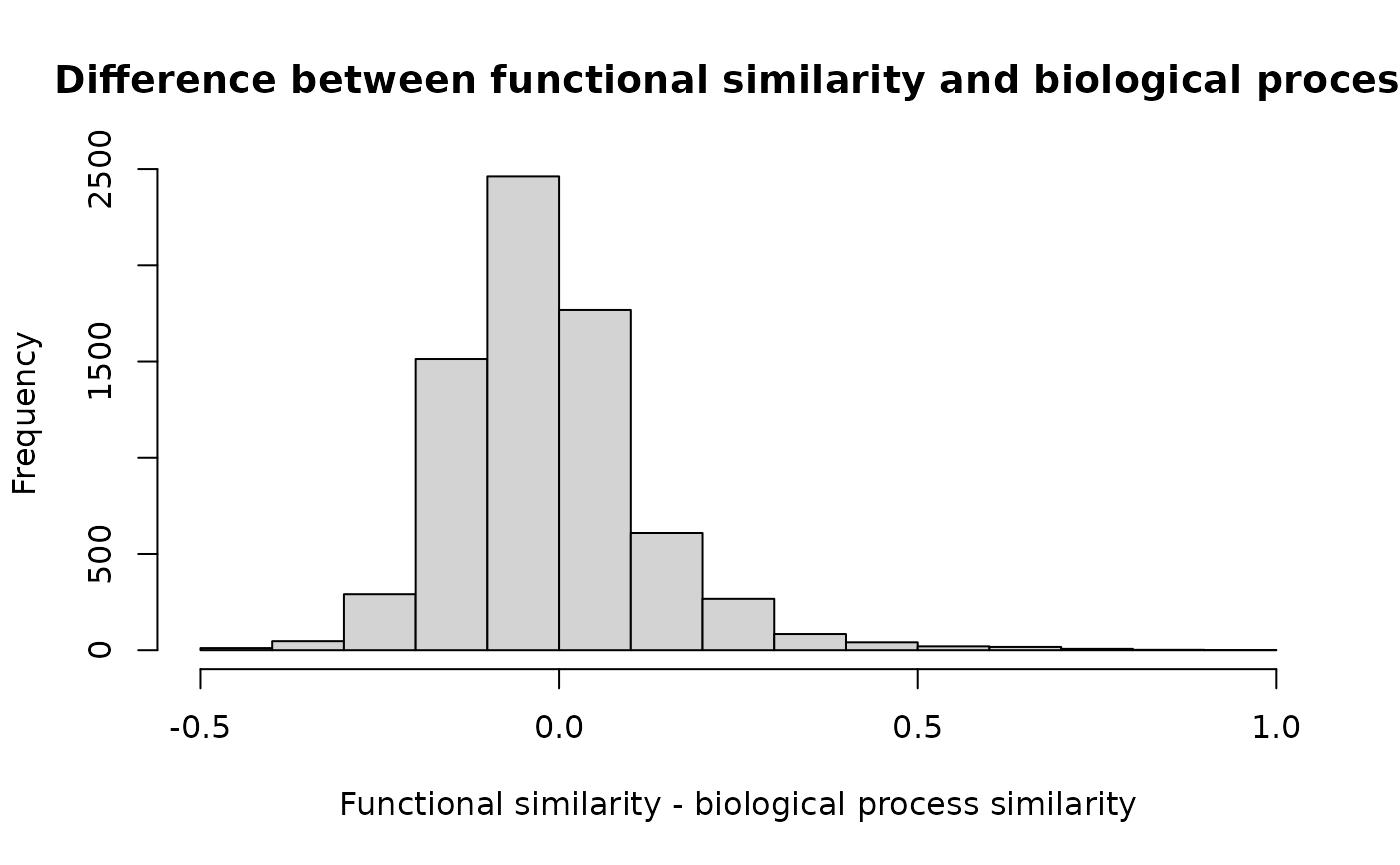
Comparison of similarities. Functional similarities compared to biological process semantic similarity.
On this graphic we can observe that some genes have a large functional similarity and few biological similarity. They are present together in several pathways while they share few biological process, indicating that they might be key elements of the pathways they are in. On the other hand some other pairs of genes show higher biological process similarity than functional similarity, indicating specialization or compartmentalization of said genes.
Session Info
sessionInfo()
## R version 4.5.1 (2025-06-13)
## Platform: x86_64-pc-linux-gnu
## Running under: Ubuntu 24.04.3 LTS
##
## Matrix products: default
## BLAS:   /usr/lib/x86_64-linux-gnu/openblas-pthread/libblas.so.3
## LAPACK: /usr/lib/x86_64-linux-gnu/openblas-pthread/libopenblasp-r0.3.26.so;  LAPACK version 3.12.0
##
## locale:
##  [1] LC_CTYPE=C.UTF-8       LC_NUMERIC=C           LC_TIME=C.UTF-8
##  [4] LC_COLLATE=C.UTF-8     LC_MONETARY=C.UTF-8    LC_MESSAGES=C.UTF-8
##  [7] LC_PAPER=C.UTF-8       LC_NAME=C              LC_ADDRESS=C
## [10] LC_TELEPHONE=C         LC_MEASUREMENT=C.UTF-8 LC_IDENTIFICATION=C
##
## time zone: UTC
## tzcode source: system (glibc)
##
## attached base packages:
## [1] stats4    stats     graphics  grDevices utils     datasets  methods
## [8] base
##
## other attached packages:
##  [1] GOSemSim_2.34.0             Hmisc_5.2-4
##  [3] boot_1.3-31                 DESeq2_1.48.2
##  [5] airway_1.28.0               SummarizedExperiment_1.38.1
##  [7] GenomicRanges_1.60.0        GenomeInfoDb_1.44.3
##  [9] MatrixGenerics_1.20.0       matrixStats_1.5.0
## [11] BioCor_1.33.3               org.Hs.eg.db_3.21.0
## [13] AnnotationDbi_1.70.0        IRanges_2.42.0
## [15] S4Vectors_0.46.0            Biobase_2.68.0
## [17] BiocGenerics_0.54.1         generics_0.1.4
## [19] BiocStyle_2.36.0
##
## loaded via a namespace (and not attached):
##  [1] DBI_1.2.3               gridExtra_2.3           GSEABase_1.70.1
##  [4] rlang_1.1.6             magrittr_2.0.4          compiler_4.5.1
##  [7] RSQLite_2.4.3           png_0.1-8               systemfonts_1.3.1
## [10] vctrs_0.6.5             reactome.db_1.92.0      stringr_1.5.2
## [13] pkgconfig_2.0.3         crayon_1.5.3            fastmap_1.2.0
## [16] backports_1.5.0         XVector_0.48.0          rmarkdown_2.30
## [19] graph_1.86.0            UCSC.utils_1.4.0        ragg_1.5.0
## [22] bit_4.6.0               xfun_0.53               cachem_1.1.0
## [25] jsonlite_2.0.0          blob_1.2.4              DelayedArray_0.34.1
## [28] BiocParallel_1.42.2     parallel_4.5.1          cluster_2.1.8.1
## [31] R6_2.6.1                bslib_0.9.0             stringi_1.8.7
## [34] RColorBrewer_1.1-3      rpart_4.1.24            jquerylib_0.1.4
## [37] Rcpp_1.1.0              bookdown_0.45           knitr_1.50
## [40] R.utils_2.13.0          base64enc_0.1-3         Matrix_1.7-3
## [43] nnet_7.3-20             rstudioapi_0.17.1       abind_1.4-8
## [46] yaml_2.3.10             codetools_0.2-20        lattice_0.22-7
## [49] KEGGREST_1.48.1         S7_0.2.0                evaluate_1.0.5
## [52] foreign_0.8-90          desc_1.4.3              Biostrings_2.76.0
## [55] BiocManager_1.30.26     checkmate_2.3.3         ggplot2_4.0.0
## [58] scales_1.4.0            xtable_1.8-4            glue_1.8.0
## [61] tools_4.5.1             data.table_1.17.8       annotate_1.86.1
## [64] locfit_1.5-9.12         fs_1.6.6                XML_3.99-0.19
## [67] grid_4.5.1              colorspace_2.1-2        GenomeInfoDbData_1.2.14
## [70] htmlTable_2.4.3         Formula_1.2-5           cli_3.6.5
## [73] rappdirs_0.3.3          textshaping_1.0.4       S4Arrays_1.8.1
## [76] gtable_0.3.6            yulab.utils_0.2.1       R.methodsS3_1.8.2
## [79] sass_0.4.10             digest_0.6.37           SparseArray_1.8.1
## [82] htmlwidgets_1.6.4       farver_2.1.2            R.oo_1.27.1
## [85] memoise_2.0.1           htmltools_0.5.8.1       pkgdown_2.1.3
## [88] lifecycle_1.0.4         httr_1.4.7              GO.db_3.21.0
## [91] bit64_4.6.0-1